Ab Initio Noise sidebands and spectra

This example demonstrates how to compute the spectra obtained from probing the system with noisy probe.

using HarmonicBalance, Plots
using ModelingToolkit, StaticArrays, StochasticDiffEq, DSP
using ModelingToolkit: setp

We first define a gelper function to compute power spectral density of the simulated response

function outputpsd(sol; fs=1.0)
    xt = getindex.(sol.u, 1)
    pxx = periodogram(
        xt; fs=fs, nfft=nextfastfft(10 * length(xt)), window=DSP.hanning, onesided=false
    )

    freqω = freq(pxx) * 2π
    perm = sortperm(freqω)
    freqlowidx = argmin(abs.(freqω[perm] .+ 0.04))
    freqhighidx = argmin(abs.(freqω[perm] .- 0.04))
    return freqω[perm][freqlowidx:freqhighidx], power(pxx)[perm][freqlowidx:freqhighidx]
end

outputpsd (generic function with 1 method)

We define the parametric oscillator using the HarmonicBalance.jl package and compute effective equations of motion at the frequency $\omega$.

@variables ω₀ γ λ F α ω t x(t)
@variables T u1(T) v1(T)

natural_equation = d(d(x, t), t) + γ * d(x, t) + (ω₀^2 - λ * cos(2 * ω * t)) * x + α * x^3
diff_eq = DifferentialEquation(natural_equation, x)

add_harmonic!(diff_eq, x, ω);
harmonic_eq = get_harmonic_equations(diff_eq)

A set of 2 harmonic equations
Variables: u1(T), v1(T)
Parameters: ω, α, γ, ω₀, λ

Harmonic ansatz: 
x(t) = u1(T)*cos(ωt) + v1(T)*sin(ωt)

Harmonic equations:

-(1//2)*u1(T)*λ + (2//1)*Differential(T)(v1(T))*ω + Differential(T)(u1(T))*γ - u1(T)*(ω^2) + u1(T)*(ω₀^2) + v1(T)*γ*ω + (3//4)*(u1(T)^3)*α + (3//4)*u1(T)*(v1(T)^2)*α ~ 0

Differential(T)(v1(T))*γ + (1//2)*v1(T)*λ - (2//1)*Differential(T)(u1(T))*ω - u1(T)*γ*ω - v1(T)*(ω^2) + v1(T)*(ω₀^2) + (3//4)*(u1(T)^2)*v1(T)*α + (3//4)*(v1(T)^3)*α ~ 0

We can compute the steady states of the system using HomotopyContinuation.jl.

ωrange = range(0.99, 1.01, 200)
fixed = Dict(ω₀ => 1.0, γ => 0.005, λ => 0.02, α => 1.0)
varied = Dict(ω => ωrange)
result = get_steady_states(harmonic_eq, TotalDegree(), varied, fixed)

plot(result; y="sqrt(u1^2 + v1^2)")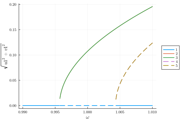

The sidebands from for the steady states will look like

sidebands1 = reduce(hcat, imag.(eigenvalues(result, 1)))'
sidebands2 = reduce(hcat, imag.(eigenvalues(result, 2)))'
scatter(ωrange, sidebands2; xlab="ω", legend=false, c=2)
scatter!(ωrange, sidebands1; xlab="ω", legend=false, c=1)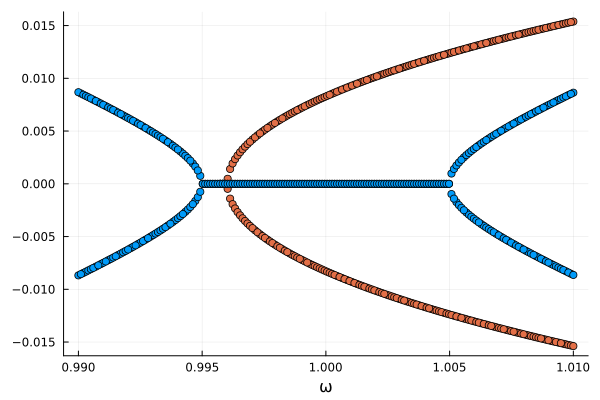

Let us now reproduce this sidebands using a noise probe. We use the ModelingToolkit extension to define the stochastic differential equation system from the harmonic equations. The resulting system will have addtivce white noise with a noise strength $\sigma =0.00005$ for each variable.

odesystem = ODESystem(harmonic_eq)
noiseeqs = [0.00005, 0.00005]  # Define noise amplitude for each variable
@mtkbuild sdesystem = SDESystem(odesystem, noiseeqs)

param = Dict(ω₀ => 1.0, γ => 0.005, λ => 0.02, α => 1.0, ω => 1.0)
Ttr = 10_000.0
T = 50_000.0
tspan = (0.0, Ttr + T)
times = range((Ttr, Ttr + T)...; step=1)

sdeproblem = SDEProblem{false}(
    sdesystem, SA[ones(2)...], tspan, param; jac=true, u0_constructor=x -> SVector(x...)
)

SDEProblem with uType StaticArraysCore.SVector{2, Float64} and tType Float64. In-place: false
timespan: (0.0, 60000.0)
u0: 2-element StaticArraysCore.SVector{2, Float64} with indices SOneTo(2):
 1.0
 1.0

Here we use StaticArrays and pass the jacobian to the integrater to speed up the computation.

Evolving the system and computing the power spectral density of the response gives

sol = solve(sdeproblem, SRA(); saveat=times)
freqω, psd = outputpsd(sol)
plot(freqω, psd; yscale=:log10, xlabel="Frequency", ylabel="Power")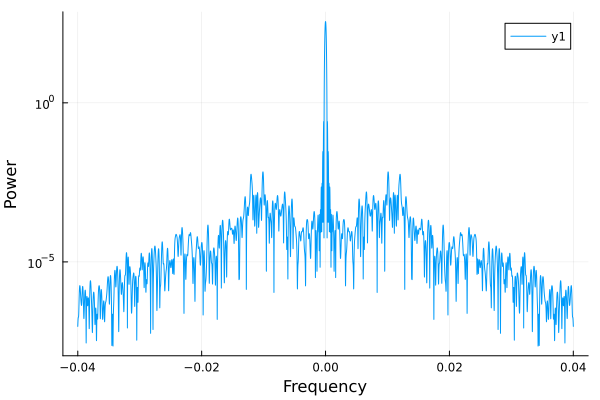

We will perform parameter sweep to generate noise spectra across the driving frequency $\omega$. For this we use the EnsembleProblem API from the SciML ecosystem.

setter! = setp(sdesystem, ω)
prob_func(prob, i, repeat) = (prob′ = remake(prob);
setter!(prob′, ωrange[i]);
prob′)
output_func(sol, i) = (outputpsd(sol), false)
prob_ensemble = EnsembleProblem(sdeproblem; prob_func=prob_func, output_func=output_func)
sol_ensemble = solve(
    prob_ensemble,
    SRA(),
    EnsembleThreads();
    trajectories=length(ωrange),
    saveat=times,
    maxiters=1e7,
)

EnsembleSolution Solution of length 200 with uType:
Tuple{Vector{Float64}, Vector{Float64}}

We find the spectrum

probe = getindex.(sol_ensemble.u, 1)[1]
spectrum = log10.(reduce(hcat, getindex.(sol_ensemble.u, 2)))
heatmap(ωrange, probe, spectrum)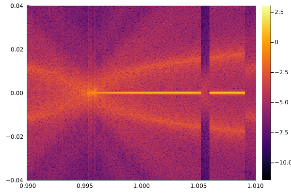

Remember that we don't do a continuation of the system, but rather initlized the system at each frequency $\omega$ and evolve it for a fixed time $T$. This leads to imperfections in the spectrum. However, if we plot the sidebands computed with HomotopyContinuation.jl on top of the spectrum, we find descent match.

heatmap(ωrange, probe, spectrum)
scatter!(ωrange, sidebands2; xlab="ω", legend=false, c=:white, markerstrokewidth=0, ms=2)
scatter!(ωrange, sidebands1; xlab="ω", legend=false, c=:black, markerstrokewidth=0, ms=2)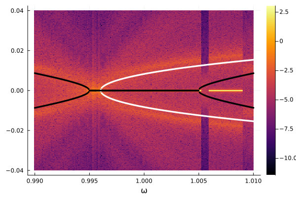

---

This page was generated using Literate.jl.