Time-dependent simulations

Most of HarmonicBalance.jl is focused on finding and analysing the steady states. Such states contain no information about transient behaviour, which is crucial to answer the following.

• Given an initial condition, which steady state does the system evolve into?

• How does the system behave if its parameters are varied in time?

It is straightforward to evolve the full equation of motion using an ODE solver. However, tracking oscillatory behaviour is computationally expensive.

In the background, we showed that nonlinear driven systems may be reduced to harmonic equations

$$\frac{d\mathbf{u}(T)}{dT}=\overline{\mathbf{F}}(\mathbf{u}),$$

As long as the chosen harmonics constituting $\mathbf{u}(T)$ capture the system's behaviour, we may numerically evolve the new effective differential equations instead of the full problem. Since the components of $\mathbf{u}(T)$ only vary very slowly (and are constant in a steady state), this is usually vastly more efficient than evolving the full problem.

Here we primarily demonstrate on the parametrically driven oscillator.

We start by defining our system.

using HarmonicBalance
@variables ω0 γ λ F θ η α ω t x(t)

eq =  d(d(x,t),t) + γ*d(x,t) + ω0^2*(1 - λ*cos(2*ω*t))*x + α*x^3 + η*d(x,t)*x^2 ~ F*cos(ω*t + θ)

diff_eq = DifferentialEquation(eq, x)
add_harmonic!(diff_eq, x, ω); # single-frequency ansatz

harmonic_eq = get_harmonic_equations(diff_eq);

A set of 2 harmonic equations
Variables: u1(T), v1(T)
Parameters: ω, α, γ, λ, ω0, η, θ, F

Harmonic ansatz: 
x(t) = u1(T)*cos(ωt) + v1(T)*sin(ωt)

Harmonic equations:

(2//1)*Differential(T)(v1(T))*ω + Differential(T)(u1(T))*γ - u1(T)*(ω^2) + u1(T)*(ω0^2) + v1(T)*γ*ω + (3//4)*(u1(T)^3)*α + (3//4)*(u1(T)^2)*Differential(T)(u1(T))*η + (1//2)*u1(T)*Differential(T)(v1(T))*v1(T)*η + (3//4)*u1(T)*(v1(T)^2)*α - (1//2)*u1(T)*λ*(ω0^2) + (1//4)*(v1(T)^2)*Differential(T)(u1(T))*η + (1//4)*(u1(T)^2)*v1(T)*η*ω + (1//4)*(v1(T)^3)*η*ω ~ F*cos(θ)

Differential(T)(v1(T))*γ - (2//1)*Differential(T)(u1(T))*ω - u1(T)*γ*ω - v1(T)*(ω^2) + v1(T)*(ω0^2) + (1//4)*(u1(T)^2)*Differential(T)(v1(T))*η + (3//4)*(u1(T)^2)*v1(T)*α + (1//2)*u1(T)*v1(T)*Differential(T)(u1(T))*η + (3//4)*Differential(T)(v1(T))*(v1(T)^2)*η + (3//4)*(v1(T)^3)*α + (1//2)*v1(T)*λ*(ω0^2) - (1//4)*(u1(T)^3)*η*ω - (1//4)*u1(T)*(v1(T)^2)*η*ω ~ -F*sin(θ)

The object harmonic_eq encodes the new effective differential equations.

We now wish to parse this input into OrdinaryDiffEq.jl and use its powerful ODE solvers. The desired object here is OrdinaryDiffEq.ODEProblem, which is then fed into OrdinaryDiffEq.solve.

Evolving from an initial condition

Given $\mathbf{u}(T_0)$, what is $\mathbf{u}(T)$ at future times?

For constant parameters, a HarmonicEquation object can be fed into the constructor of ODEProblem. The syntax is similar to DifferentialEquations.jl :

using OrdinaryDiffEq
x0 = [0.; 0.] # initial condition
fixed = (ω0 => 1.0, γ => 1e-2, λ => 5e-2, F => 1e-3,  α => 1.0, η => 0.3, θ => 0, ω => 1.0) # parameter values

ode_problem = ODEProblem(harmonic_eq, fixed, x0 = x0, timespan = (0,1000))

ODEProblem with uType Vector{Float64} and tType Int64. In-place: true
timespan: (0, 1000)
u0: 2-element Vector{Float64}:
 0.0
 0.0

OrdinaryDiffEq.jl takes it from here - we only need to use solve.

time_evo = solve(ode_problem, saveat=1.0);
plot(time_evo, ["u1", "v1"], harmonic_eq)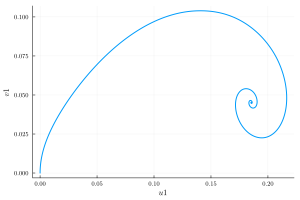

Running the above code with x0 = [0.2, 0.2] gives the plots

x0 = [0.2; 0.2] # initial condition
ode_problem = remake(ode_problem, u0 = x0)
time_evo = solve(ode_problem, saveat=1.0);
plot(time_evo, ["u1", "v1"], harmonic_eq)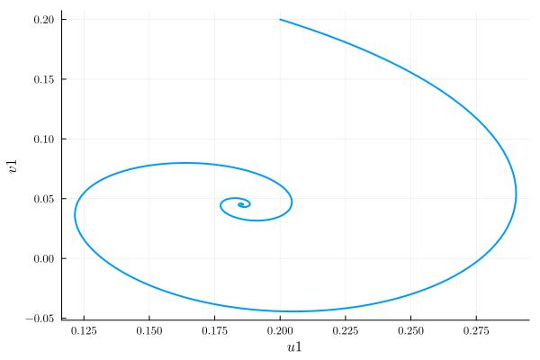

Let us compare this to the steady state diagram.

varied = ω => range(0.9, 1.1, 100)
result = get_steady_states(harmonic_eq, varied, fixed)
plot(result, "sqrt(u1^2 + v1^2)")

Clearly when evolving from x0 = [0.,0.], the system ends up in the low-amplitude branch 2. With x0 = [0.2, 0.2], the system ends up in branch 3.

Adiabatic parameter sweeps

Experimentally, the primary means of exploring the steady state landscape is an adiabatic sweep one or more of the system parameters. This takes the system along a solution branch. If this branch disappears or becomes unstable, a jump occurs.

The object ParameterSweep specifies a sweep, which is then used as an optional sweep keyword in the ODEProblem constructor.

sweep = ParameterSweep(ω => (0.9,1.1), (0, 2e4))

ParameterSweep(Dict{Num, Function}(ω => TimeEvolution.var"#f#1"{Tuple{Float64, Float64}, Float64, Int64}((0.9, 1.1), 20000.0, 0)))

The sweep linearly interpolates between $\omega =0.9$ at time 0 and $\omega =1.1$ at time 2e4. For earlier/later times, $\omega$ is constant.

Let us now define a new ODEProblem which incorporates sweep and again use solve:

ode_problem = ODEProblem(harmonic_eq, fixed, sweep=sweep, x0=[0.1;0.0], timespan=(0, 2e4))
time_evo = solve(ode_problem, saveat=100)
plot(time_evo, "sqrt(u1^2 + v1^2)", harmonic_eq)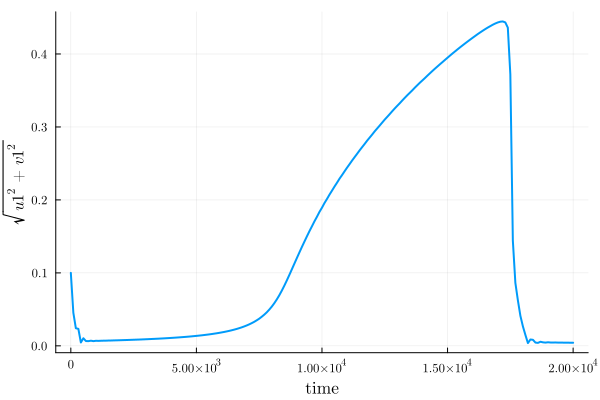

We see the system first evolves from the initial condition towards the low-amplitude steady state. The amplitude increases as the sweep proceeds, with a jump occurring around $\omega =1.08$ (i.e., time 18000).